- Real eigenvalues
- Eigenvectors can be chosen orthonormal
Usual case
\[ \textbf{A} = \textbf{S}\Lambda\textbf{S}^{-1} \]Symmetric case
\[ \textbf{A} = \textbf{Q}\Lambda\textbf{Q}^{-1} = \textbf{Q}\Lambda\textbf{Q}^{T} \]Spectral theorem
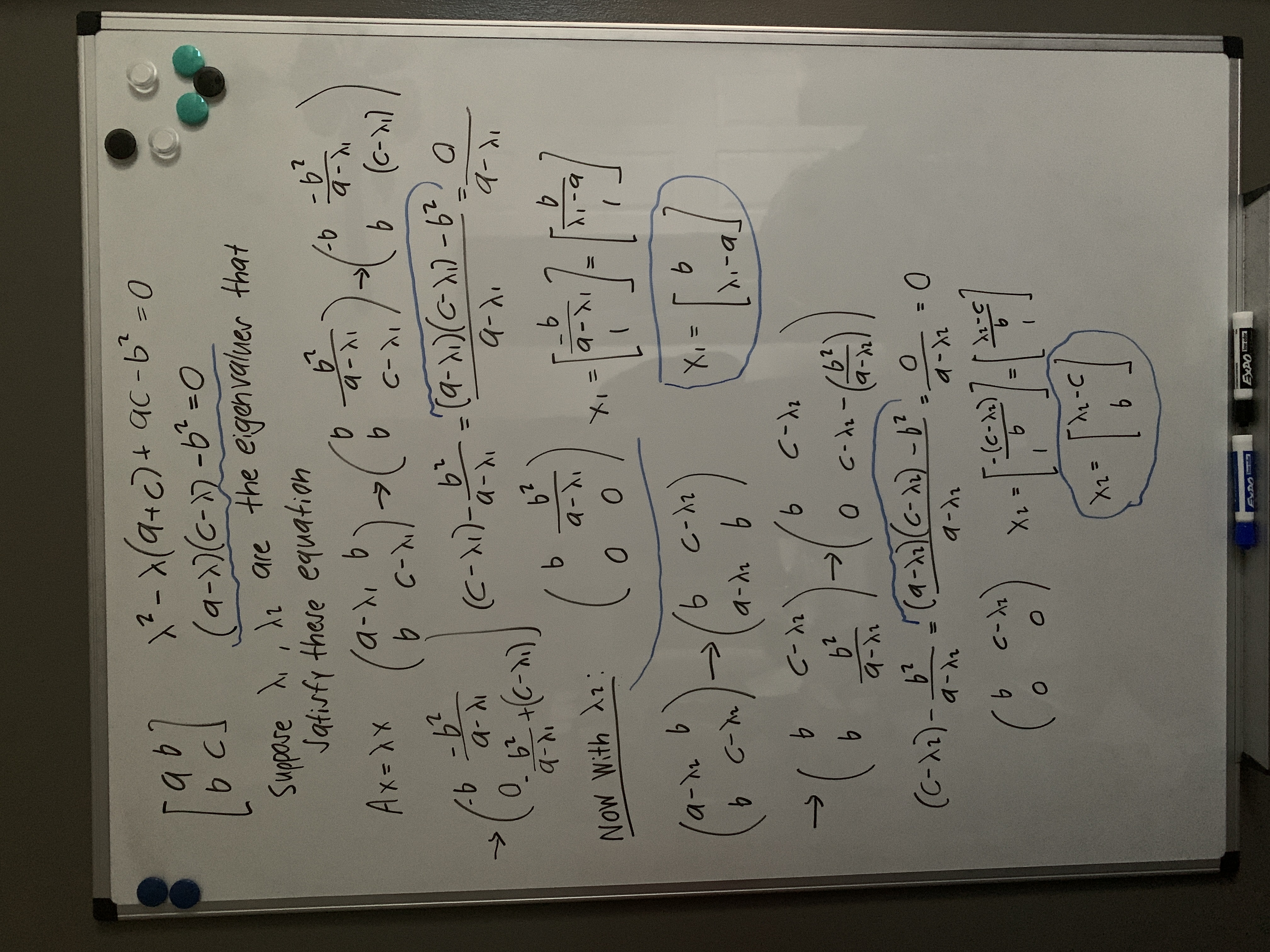
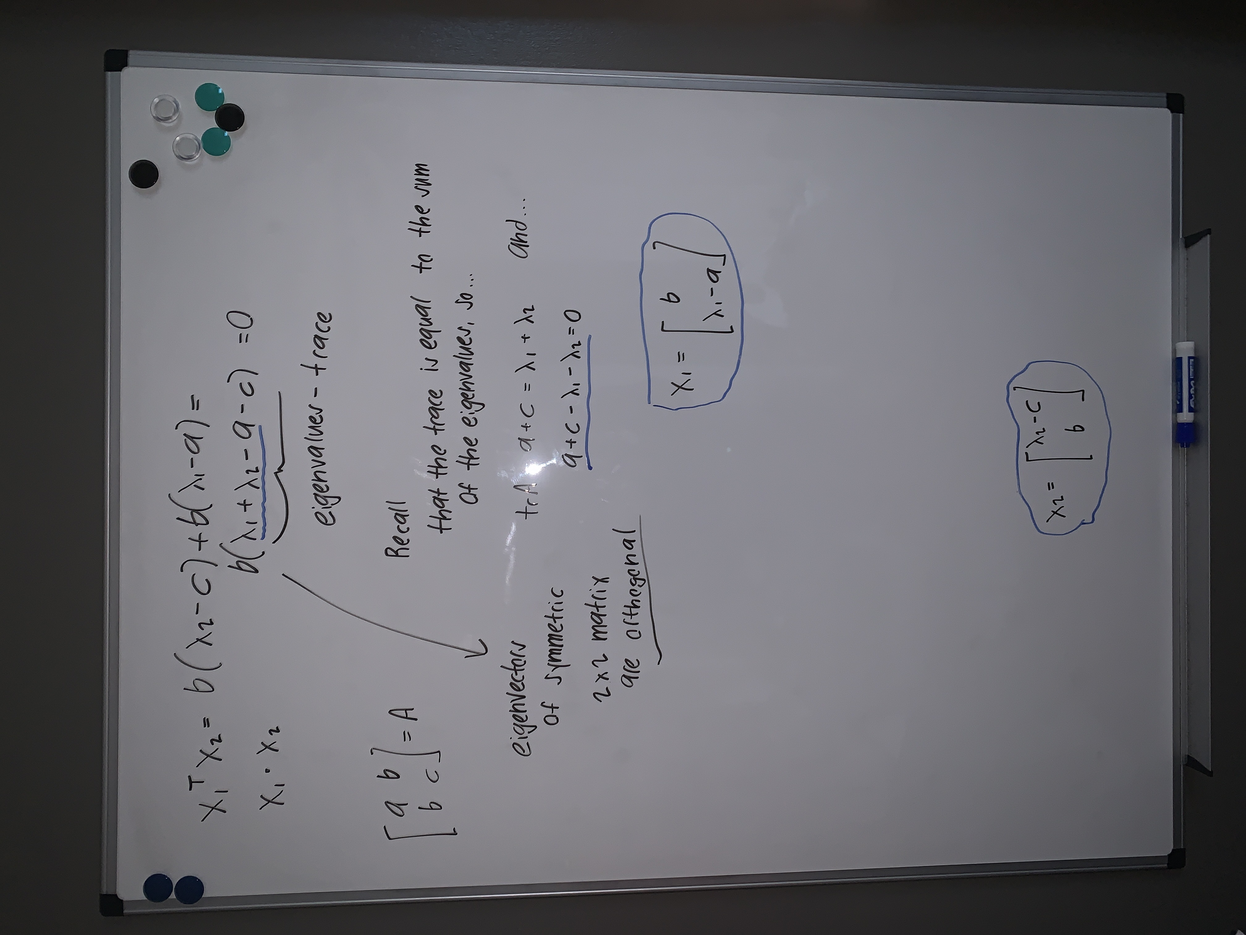
This only shows the 2 by 2 case.
\[ \textbf{A} = \sum_{i=0}^{n} \lambda_{i}x_{i}x_{i}^{T} = \lambda_{1}x_{1}x_{1}^{T} + \lambda_{2}x_{2}x_{2}^{T} + \cdots + \lambda_{n}x_{n}x_{n}^{T} \]
We see that \(\textbf{A}\) is equal a sum of projections matrices where they are projecting onto eigenspaces. In other words, spectral theorem says that symmetric matrices can be expressed as a combination of projection matrices.
\[ \textbf{A} = \lambda_{1}\textbf{P}_{1} + \lambda_{2}\textbf{P}_{2} + \cdots + \lambda_{n}\textbf{P}_{n} \] where \( \textbf{P}_{i} = x_{i}x_{i}^{T} \)\[ \textbf{A}v = (\lambda_{1}\textbf{P}_{1} + \lambda_{2}\textbf{P}_{2} + \cdots + \lambda_{n}\textbf{P}_{n})v = \lambda_{1}\textbf{P}_{1}v + \lambda_{2}\textbf{P}_{2}v + \cdots + \lambda_{n}\textbf{P}_{n}v \]
Antisymmetric matrices have pure imaginary eigenvalues.
Proof:
Let \(\textbf{A}\) be an \(n\) by \(n\) antisymmetric matrix.
By definition,
\[ \textbf{A}^{T} = -\textbf{A} \]Suppose \(\lambda\) is an eigenvalue of \(\textbf{A}\) and \(x\) is the corresponding eigenvector.
\[ \textbf{A}x = \lambda x \] \[ \textbf{A}^{T}\textbf{A}x = \lambda\textbf{A}^{T}x \] \[ \textbf{A}^{T}\textbf{A}x = -\textbf{A}^{2}x = -\lambda(\lambda)x = -\lambda^{2}x \]The matrix \(\textbf{A}^{T}\textbf{A}\) is positive semi-definite and \(-\lambda^{2}\) is an eigenvalue of \(\textbf{A}^{T}\textbf{A}\).
So, by definition of positive semi-definite matrices,
\[ -\lambda^{2} \geq 0 \] \[ \lambda^{2} \leq 0 \]The only numbers that have squares less than zero are imaginary numbers. This tells us that \(\lambda\) must have the imaginary unit \(i\) and therefore
\[ \lambda = bi \] for \(b\in \mathbb{R}\)Q.E.D.
Suppose we have a column vector \(z\) with complex components \(z_{1}, z_{2}, \ldots, z_{n}\).
\[ z = \begin{bmatrix} z_{1} \\ z_{2} \\ \vdots \\ z_{n} \end{bmatrix} \]How do we find the length squared? Normally with real vectors, we simply take the dot product of that vector with itself. To find the length squared of \(z\), we take the dot product of it with its conjugate. This is analogous to finding the absolute value (or modulus) of a complex number.
\[ ||z||^{2} = \bar{z}^{T}z \]If we want just the length, then we take the square root.
\[ ||z|| = \sqrt{||z||^{2}} \]There is a way that express the transpose and the complex conjugate of a vector at once.
\[ \overline{z^{T}} = z^{H} \]read as z "hermitation".
Hermite, Hermitation
The inner product changes too.
Hermitian Matrices
\[ \textbf{A}^{H} = \textbf{A} \]Unitary
Example:
Find the length squared of the vector \((1, i)\).
\[ \begin{bmatrix} 1 & -i \end{bmatrix} \begin{bmatrix} 1 \\ i \end{bmatrix} = 1 + -i(i) = 1 + 1 = 2\]The length is then consequently equal to \(\sqrt{2}\).
\[ (a + bi)(a - bi) = a^{2} + b^{2} \]
The Discrete Fourier Transform and its optimized version, the Fast Fourier Transform, have matrix representations that happen to be complex. Brief notes on them here.
There are multiple tests that we can use to determine whether or not a matrix is positive definite.
- All the eigenvalues are positive. \[ \lambda_{1} > 0 \quad \lambda_{2} > 0 \quad \cdots \quad \lambda_{n} > 0 \]
- Subdeterminants are greater than 0.
- All the pivots are positive.
- \( f(x_{1}, x_{2}, \ldots, x_{n}) = x^{T}\textbf{A}x > 0\) for all \(x \neq 0\)
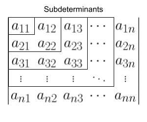
The function \(f\) will always be the equation of a quadratic surface.
As usual, we will do an example with the 2 by 2 case.
\[ \textbf{A} = \begin{bmatrix} a & b \\ b & c \end{bmatrix} \]Here are the different tests that we can use:
- Positive eigenvalues \(\lambda_{1} > 0 \quad \lambda_{2} > 0\).
- Positive subdeterminants: \[ a > 0 \quad \textrm{and} \quad \begin{vmatrix} a & b \\ b & c \end{vmatrix} > 0 \]
- Positive pivots: \[a > 0 \quad \textrm{and} \quad \frac{ac-b^{2}}{a}\]
- \( v^{T}\textbf{A}v > 0\) for all \(x \neq 0\) \[ \begin{bmatrix} v_{1} & v_{2} \end{bmatrix} \begin{bmatrix} a & b \\ b & c \end{bmatrix} \begin{bmatrix} v_{1} \\ v_{2} \end{bmatrix} > 0 \] \[ \begin{bmatrix} v_{1} & v_{2} \end{bmatrix} \begin{bmatrix} av_{1} + bv_{2} \\ bv_{1} + cv_{2} \end{bmatrix} = av_{2}^{2} + 2bv_{1}v_{2} + cv_{2}^{2} > 0 \]
Let \(v_{1} = x\) and \(v_{2} = y\)
\[ f(x, y) = ax^{2} + 2bxy + cy^{2} > 0 \]This is where calculus comes into play. Derivatives can be used to determine if the function is ever negative. If so, then the matrix is not positive definite. Recall the first and second derivative test for finding the extrema of a function. That is what we can use in this situation.
One way that we can figure out if the function is always positive is by completing the square. This leaves us with a sum of squares. Squaring a real number always yields a positive.
\[ ax^{2} + 2bxy + cy^{2} = a\left(x^{2} + \frac{2bxy}{a} + \frac{cy^{2}}{a}\right) = a\left(x + \frac{by}{a}\right)^{2} + \left(c - \frac{b^{2}}{a}\right)y^{2} \] \[ = a\left(x + \frac{by}{a}\right)^{2} + \det(\textbf{A})y^{2} \]If any of the terms are negative, then \(\textbf{A}\) is not positive definite. The coefficient of each term represents a pivot. The inner coefficient for the \(y\) term represents the multipliers. This all goes back to Gauss-Jordan elimination.
Minimum:
First derivative = 0
\( \frac{du}{dx} = 0 \)Second derivative > 0 to confirm that the critical point is a minimum.
\( \frac{d^{2}u}{dx^{2}} = 0 \)The matrix of second partial derivatives must have a positive determinant for there to be a maximum/minimum. If it is positive definite, it is a minimum.
When the determinant is negative, there is a saddle point. If the determinant is 0, then the second partial derivative test is inconclusive and more information is needed to classify the critical point.
Hessian matrix
\[ \textbf{H}_{f} = \begin{bmatrix} f_{xx} & f_{xy} \\ f_{yx} & f_{yy} \end{bmatrix} \]Know that \(f_{xy} = f_{yx}\).
\[ \det\textbf{H}_{f} = f_{xx}f_{yy} - [f_{xy}]^{2} \]Principle Axis Theorem
The eigenvalues and eigenvectors tell us the direction and length of the principle axes.
Use spectral theorem
\[ v^{T}\textbf{A}v = v^{T}\left(\sum_{i=1}^{n} \lambda_{i}x_{i}x_{i}^{T}\right)v = \sum_{i=1}^{n} \lambda_{i}v^{T}x_{i}x_{i}^{T}v = \sum_{i=1}^{n} \lambda_{i}(x_{i}^{T}v)^{T}x_{i}^{T}v = \sum_{i=1}^{n} \lambda_{i} \ ||x_{i}v||^{2} \]The magnitude of a nonzero vector is always greater than 0. If all the eigenvalues \(\lambda_{1}, \lambda_{2}, \ldots, \lambda_{n}\) are positive, then
\[ v^{T}\textbf{A}v = \sum_{i=1}^{n} \lambda_{i} \ ||x_{i}v||^{2} > 0 \]Related to the idea of positive definiteness, there are other similar categorizations of matrices: positive semi-definite, negative definite, and negative semi-definite.
Theorem
The sum of two positive definite matrices is positive definite.
Proof:
Suppose \(\textbf{A}\) and \(\textbf{B}\) are two positive definite matrices.
By definition
\[ x^{T}\textbf{A}x > 0 \qquad x^{T}\textbf{B}x > 0 \] for all \(x\neq\vec{0}\)It follows that
\[ x^{T}\textbf{A}x + x^{T}\textbf{B}x = x^{T}(\textbf{A} + \textbf{B})x > 0 \]and thus \(\textbf{A} + \textbf{B}\) is positive definite concluding that the sum of two positive definite matrices is also positive definite.
Q.E.D.
Theorem
Given an \(m\) by \(n\) matrix \(\textbf{A}\), if \(\textrm{rank}(\textbf{A}) = n\) then \(\textbf{A}^{T}\textbf{A}\) is positive definite.
Proof:
Suppose \(\textbf{A}\) is an \(m\) by \(n\) matrix with \(\textrm{rank}(\textbf{A}) = n\).
\(\textbf{A}^{T}\textbf{A}\) is square and symmetric.
\[ x^{T}\textbf{A}^{T}\textbf{A}x = (\textbf{A}x)^{T}\textbf{A}x = ||\textbf{A}x||^{2} \]The magntitude of a vector is always nonnegative. This shows
\[ ||\textbf{A}x||^{2} \geq 0 \]Recall that for all matrices, the sum of dimension of its nullspace and the dimension of its column space add to its number of columns.
\[ \dim(C(\textbf{A})) + \dim(N(\textbf{A})) = n \]But the rank of \(\textbf{A}\) is equal to the number of columns.
\[ \textrm{rank}(\textbf{A}) = n \]As a result of this, \(\textbf{A}\) has \(n\) linearly independent columns and
\[ \dim(C(\textbf{A})) = n \]showing
\[ \dim(N(\textbf{A})) + n = n \qquad \Rightarrow \qquad \dim(N(\textbf{A})) = 0 \]The only vector that satisfies the equation
\[ ||\textbf{A}x||^{2} = 0 \]is the zero vector. It has no nontrivial solutions. This means previous equation
\[ ||\textbf{A}x||^{2} \geq 0 \]can be rewritten as
\[ ||\textbf{A}x||^{2} > 0 \]
finally proving that
\[ x^{T}\textbf{A}^{T}\textbf{A}x > 0 \]By the definition of positive matrices, \(\textbf{A}^{T}\textbf{A}\) is positive definite (as was to be shown).
Q.E.D.
Theorem
The inverse of a positive definite matrix is positive definite.
Two \(n\) by \(n\) matrices \(\textbf{A}\) and \(\textbf{B}\) are similar if
\[ \textbf{B} = \textbf{M}^{-1}\textbf{A}\textbf{M} \] for some \(n\) by \(n\) matrix \(\textbf{M}\)With matrix diagonalization, similar matrices are produced.
\[ \Lambda = \textbf{S}^{-1}\textbf{A}\textbf{S} \]\(\textbf{A}\) is similar to \(\Lambda\).
Similar matrices have the same eigenvalues. All matrices with matching eigenvalues and belong to this "family" of matrices.
\[ \textbf{B}x = \lambda x \] \[ \textbf{M}^{-1}\textbf{A}\textbf{M}x = \lambda x \] \[ \textbf{A}(\textbf{M}x) = \lambda (\textbf{M}x) \]Having the same eigenvalues implies that the matrices also have the same trace and determinant. Finding similar matrices can be reduced to finding matrices that preserve this property.
Example:
\[ \begin{bmatrix} 4 & 1 \\ 0 & 4 \end{bmatrix}, \begin{bmatrix} 5 & 1 \\ -1 & 3 \end{bmatrix}, \begin{bmatrix} 4 & 0 \\ 17 & 4 \end{bmatrix}, \begin{bmatrix} 2 & 2 \\ -2 & 6 \end{bmatrix} \]All four of these matrices have a trace of 8 and determinant of 16.
Similar matrices also have the same number of independent eigenvectors. This stems from the fact that they have the same eigenvalues.
Jordan Matrix/Jordan Form
Jordan Blocks
The Jordan form is the most diagonal matrix in the family.
How do we find \(\textbf{U}\) and \(\textbf{V}\)?
Remember that \(\textbf{A}^{T}\textbf{A}\) is positive definite.
\[ \textbf{A}^{T}\textbf{A} = (\textbf{U}\Sigma\textbf{V}^{T})^{T} \textbf{U}\Sigma\textbf{V}^{T} \] \[ = \textbf{V}\Sigma^{T}\textbf{U}^{T}\textbf{U}\Sigma\textbf{V}^{T} \]Recall that orthogonal matrices have the property that the inverse of an orthogonal matrix is equal to its transpose. Diagonal matrices, on the other hand, have that they are equal to their transpose. Following this
\[ \textbf{U}^{T} = \textbf{U}^{-1} \quad \textrm{and} \quad \Sigma^{T} = \Sigma \]Applying this to the equation above
\[ \textbf{A}^{T}\textbf{A} = \textbf{V}\Sigma\textbf{U}^{-1}\textbf{U}\Sigma\textbf{V}^{T} \] \[ = \textbf{V}\Sigma^{2}\textbf{V}^{T} \]The product of \(\textbf{A}^{T}\textbf{A}\) will be positive semi-definite. In other words, the eigenvalues will be greater than or equal to 0. With symmetric matrices, there was the following factorization:
\[ \textbf{A} = \textbf{Q}\Lambda\textbf{Q}^{T} \]This is telling us that \(\textbf{V}\) will be the matrix of eigenvectors belonging to \(\textbf{A}^{T}\textbf{A}\) and \(\Sigma\) will have the positive square roots of the eigenvalues.
A similar process can be used to find the value of \(\textbf{U}\).
\[ \textbf{A}\textbf{A}^{T} = \textbf{U}\Sigma\textbf{V}^{T}(\textbf{U}\Sigma\textbf{V}^{T})^{T} \] \[ = \textbf{U}\Sigma\textbf{V}^{T}\textbf{V}\Sigma^{T}\textbf{U}^{T} \] \[ = \textbf{U}\Sigma\textbf{V}^{-1}\textbf{V}\Sigma\textbf{U}^{T} \] \[ = \textbf{U}\Sigma^{2}\textbf{U}^{T} \]Note: \(\Sigma^{T} = \Sigma\) on the condition that it is a square diagonal matrix.
\[ \textbf{A}\textbf{V} = \textbf{U}\Sigma \]
Linear transformations, also called mappings, are a way to visually view the effects of matrices.
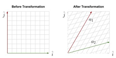
The transformation shown above maps vectors in \(\mathbb{R}^{2}\) to other vectors in \(\mathbb{R}^{2}\). The two vectors \(a_{1}\) and \(a_{2}\) form a basis for \(\mathbb{R}^{2}\) as they are linearly independent. So do the standard basis vectors.
The matrix that represents this transformation is 2 by 2.
\[ \textbf{A} = \begin{bmatrix} & \\ a_{1} & a_{2} \\ & \end{bmatrix} \]Functions are exactly like. For instance, say we have a function \(f\) of two inputs \(x\) and \(y\). The function maps the two inputs to a single output that we will call \(z\). In calculus, the relationship is expressed as follows:
\[ z = f(x, y) \qquad f: \mathbb{R}^{2} \rightarrow \mathbb{R} \]Every linear transformation has a matrix. How do we find it?
Example 1: Projection
Linear transformations have the following two properties:
Given a linear transformation \(T\) and two vectors \(v\) and \(w\),
- \[ T(v+w) = T(v) + T(w) \]
- \[ T(cv) = cT(w) \] where \(c\) is some constant
The second property immediately implies an important fact about linear transformations (emphasis on the linear).
\[ T(0) = 0 \]The zero vector must remain fixed for a transformation to be considered linear.
Example 2: Rotation
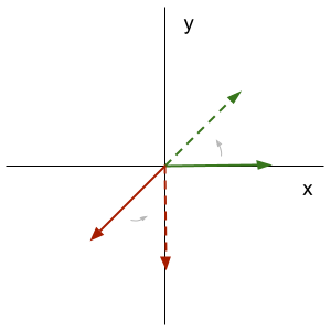
45 degree counter-clockwise rotation matrix:
\[ \textbf{R}\left(\frac{\pi}{4}\right) = \begin{bmatrix} \frac{\sqrt{2}}{2} & - \frac{\sqrt{2}}{2} \\ \frac{\sqrt{2}}{2} & \frac{\sqrt{2}}{2} \end{bmatrix} \] \[ \begin{bmatrix} \frac{\sqrt{2}}{2} & - \frac{\sqrt{2}}{2} \\ \frac{\sqrt{2}}{2} & \frac{\sqrt{2}}{2} \end{bmatrix} \begin{bmatrix} \frac{\sqrt{2}}{2} & - \frac{\sqrt{2}}{2} \\ \frac{\sqrt{2}}{2} & \frac{\sqrt{2}}{2} \end{bmatrix} = \begin{bmatrix} 0 & -1 \\ 1 & 0 \end{bmatrix} \]Applying the transformation twice is equivalent to performing a single 90 degree rotation. This showcases the fact that matrix multiplication can be thought of as the composition of transformations.
\[ \textbf{R}\left(\frac{\pi}{4}\right)^{2} = \textbf{R}\left(\frac{\pi}{2}\right) \]Example 3: Reflection about the \(x\)-axis
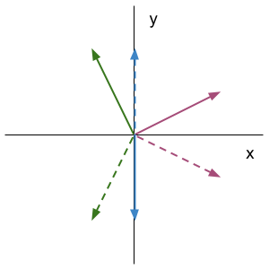
Example 4: House
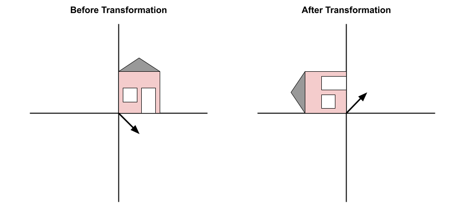
Transformations act on all points in space at once. The house can be thought of as a connection of multiple vectors. This specific transformation performs a 90 degree rotation on all vectors in the plane.
\[ T = \textbf{A} \]
Choosing an eigenvector basis—eigenbasis—leads to the diagonal matrix \(\Lambda\) of eigenvalues.
The number of input vectors is \(n\), the number of columns, and the number of output vectors is \(m\), the number of rows.
\[ T: \mathbb{R}^{n} \rightarrow \mathbb{R}^{m} \]Example:
Define a transformation \(\textbf{J}\) such that
\[ J: \mathbb{R}^{3} \rightarrow \mathbb{R}^{2} \] \[ J = \textbf{B} \] \[ \textbf{B}x = v \] \[ = \begin{bmatrix} b_{11} & b_{12} & b_{13} \\ b_{21} & b_{22} & b_{23} \end{bmatrix} \begin{bmatrix} x_{1} \\ x_{2} \\ x_{3} \end{bmatrix} = \begin{bmatrix} v_{1} \\ v_{2} \end{bmatrix} \] \[ [2\times 3] \times [3\times 1] = [2\times 1] \]With this example, the matrix \(\textbf{B}\) maps the input vector \(x \in\mathbb{R}^{3} \) to the output vector \(v \in\mathbb{R}^{2} \).
How much information do we need to find the matrix for a linear transformation?
You need \(n\) independent vectors in \(\mathbb{R}^{n}\) to represent all vectors \(v\in\mathbb{R}^{n}\).
\[ a_{1}, a_{2}, \ldots, a_{n} \]These are the input vectors. All vectors in \(\mathbb{R}^{n}\) can be expressed as a combination of these basis vectors.
\[ v = c_{1}a_{1} + c_{2}a_{2} + \cdots + c_{n}a_{n} \] for some constants \(c_{1}, c_{2}, \ldots, c_{n}\)If I know what the linear transformation does to the basis vectors, then I also know what it does to all the linear combinations of the basis vectors. This all extends from the properties of linear transformations.
What we need to know:
\[ T(a_{1}), T(a_{2}), \ldots, T(a_{n}) \]It tells us that for any vector \(v\):
\[ T(v) = c_{1}T(a_{1}) + c_{2}T(a_{2}) + \cdots + c_{n}T(a_{n}) \]\(c_{1}, c_{2}, \ldots, c_{n}\) are the coordinates given by the input vector.
\[ x = \begin{bmatrix} c_{1} \\ c_{2} \\ \vdots \\ c_{n} \end{bmatrix} \]So if you know what the transformation does to every vector in a basis, then you know what the transformation does to every vector in the space.
Steps to finding the matrix for a linear transformation:
- Choose an input basis
- Choose an output basis
- Determine the appropriate values that map the input vectors to the output vectors
Given inputs \(v_{1}, v_{2}, \ldots, v_{n}\) and outputs \(w_{1}, w_{2}, \ldots, w_{n}\)
The first column is given by \(T(v_{1})\), the second column is given by \(T(v_{2})\) and so on.
\[ T(v_{1}) = a_{11}w_{1} + a_{21}w_{2} + \cdots + a_{m1}w_{m} \\ T(v_{2}) = a_{12}w_{1} + a_{22}w_{2} + \cdots + a_{m2}w_{m} \\ \vdots \\ T(v_{n}) = a_{1n}w_{1} + a_{2n}w_{2} + \cdots + a_{mn}w_{mn} \]\[ \textbf{A}(\textrm{Input Coordinates}) = (\textrm{Ouput Coordinates})\]
Oftentimes with transformations, the standard basis is treated as the input basis.
The standard basis vectors for \(\mathbb{R}^{3}\):
\[ \begin{bmatrix} 1 \\ 0 \\ 0 \end{bmatrix} \qquad \begin{bmatrix} 0 \\ 1 \\ 0 \end{bmatrix} \qquad \begin{bmatrix} 0 \\ 0 \\ 1 \end{bmatrix} \]Example 5: Calculating Derivatives
Believe it or not, differentiation is a linear operation which means that it can be represented as a linear transformation.
\[ \begin{align} \frac{d}{dx}(ax^{2} + bx + c) &= \frac{d}{dx}(ax^{2}) + \frac{d}{dx}(bx) + \frac{d}{dx}(c) \\ &= a\frac{d}{dx}(x^{2}) + b\frac{d}{dx}(x) + c\frac{d}{dx}(1) \\ &= a(2x) + b \end{align} \]This means there exists a transformation for differentiation.
\[ \textbf{A}: \mathbb{R}^{3} \rightarrow \mathbb{R}^{2} \] \[ \textbf{A} = \frac{d}{dx} \]Say we have a general quadratic
\[ f(x) = ax^{2} + bx + c \]The input basis will be
\[ \left\{ \begin{bmatrix} x^{2} \\ 0 \\ 0 \end{bmatrix}, \begin{bmatrix} 0 \\ x \\ 0 \end{bmatrix}, \begin{bmatrix} 0 \\ 0 \\ 1 \end{bmatrix} \right\} \]and the output basis will be
\[ \left\{ \begin{bmatrix} x \\ 0 \end{bmatrix}, \begin{bmatrix} 0 \\ 1 \end{bmatrix} \right\} \]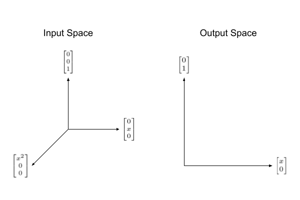
The matrix that differentiates this function would look as follows:
\[ \textbf{A} = \begin{bmatrix} 2 & 0 & 0 \\ 0 & 1 & 0 \end{bmatrix} \]The computation would work out nicely.
\[ \textbf{A}f = \begin{bmatrix} 2 & 0 & 0 \\ 0 & 1 & 0 \end{bmatrix} \begin{bmatrix} a \\ b \\ c \end{bmatrix} = \begin{bmatrix} 2a \\ b \end{bmatrix} \]Referring back to the output basis, this is really
\[ \begin{bmatrix} 2ax \\ b \end{bmatrix} \]There we go! We have a transformation that takes derivatives of polynomials.
\[ \textbf{A}f = f' \]There is one last fact that I will mention, not specific to this problem. The inverse matrix gives the inverse to the transformation. With the above example, the inverse of differentiation is integration.
There are two kinds of image compression: lossless and lossy compression.
Images can be represented as vectors as follows:
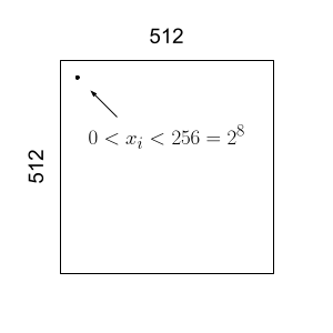
This image is 512 pixels by 512 pixels.
That means that the vector containing this information, we will call \(x\), has \(512^{2}\) components. That is an enormous amount of information.
\[ x \in \mathbb{R}^{n} \] where \(n=512^{2}\)Each pixel has a grayscale. That grayscale is typically a value between 0 and 255.
The ith pixel has a value
\[ 0 \leq x_{i} < 256 \]There are \(2^{9}\) possible values that each pixel can have. If we introduce color in the form of RGB, the dimension of the vector becomes \(n=3(512^{2})\). Why? RBG values consist of three numbers that range from 0 to 255. One value is for the green scale, another for the blue scale, and one more for the red scale.
Here is an example of how the signal may look:
\[ x = \begin{bmatrix} \vdots \\ 121 \\ 124 \\ \vdots \end{bmatrix} \]If this is a black and white image, then the grayscale is used and there are \(512^{2}\) entries.
JPEG — Joint Photographic Experts Group
By default, images use the standard basis:
\[ \begin{bmatrix} 1 \\ 0 \\ 0 \\ \vdots \\ 0 \end{bmatrix} \quad \begin{bmatrix} 0 \\ 1 \\ 0 \\ \vdots \\ 0 \end{bmatrix} \quad \cdots \quad \begin{bmatrix} 0 \\ 0 \\ 0 \\ \vdots \\ 1 \end{bmatrix} \]We want to use a better basis. Two popular choices are the Fourier basis and the wavelet basis.
Often 8 by 8 is a good choice. There will be 64 coeffficents for pixels in each.
How does that affect the 256 by 256 image?
Here is the 8 by 8 Fourier basis:
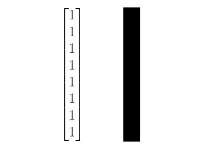
\[ \left\{ \begin{pmatrix} 1 \\ 1 \\ 1 \\ 1 \\ 1 \\ 1 \\ 1 \\ 1 \end{pmatrix}, \begin{pmatrix} 1 \\ \omega \\ \omega^{2} \\ \omega^{3} \\ \omega^{4} \\ \omega^{5} \\ \omega^{6} \\ \omega^{7} \end{pmatrix}, \cdots \right\} \]Here is the 8 by 8 wavelet basis:
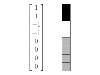
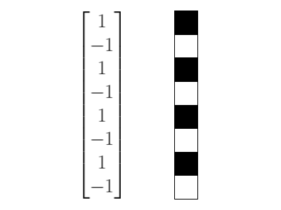
\[ \left\{ \begin{pmatrix} 1 \\ 1 \\ 1 \\ 1 \\ 1 \\ 1 \\ 1 \\ 1 \end{pmatrix}, \begin{pmatrix} 1 \\ 1 \\ 1 \\ 1 \\ -1 \\ -1 \\ -1 \\ -1 \end{pmatrix}, \begin{pmatrix} 1 \\ 1 \\ -1 \\ -1 \\ 0 \\ 0 \\ 0 \\ 0 \end{pmatrix}, \begin{pmatrix} 0 \\ 0 \\ 0 \\ 0 \\ 1 \\ 1 \\ -1 \\ -1 \end{pmatrix}, \begin{pmatrix} 1 \\ -1 \\ 0 \\ 0 \\ 0 \\ 0 \\ 0 \\ 0 \end{pmatrix}, \begin{pmatrix} 0 \\ 0 \\ 1 \\ -1 \\ 0 \\ 0 \\ 0 \\ 0 \end{pmatrix}, \begin{pmatrix} 0 \\ 0 \\ 0 \\ 0 \\ 1 \\ -1 \\ 0 \\ 0 \end{pmatrix}, \begin{pmatrix} 0 \\ 0 \\ 0 \\ 0 \\ 0 \\ 0 \\ 1 \\ -1 \end{pmatrix} \right\} \]Notice that with both of these matrices, they can represent every vector in \(\mathbb{R}^{8}\).
The first vector is completely solid. Taking a combination of the last four vectors, we get almost like a checkboard pattern. That vector has the highest frequency.
What makes a basis good?
Firstly, its matrix must be fast to compute. For instance, with the Fourier basis, there is the FFT. The wavelet basis has the fast wavelet transform. What makes the wavelet matrix fast to compute? It is an orthogonal basis. It can easily be made to be orthonormal by dividing each basis vector by the length.
The first two would be divided by \(\frac{1}{\sqrt{8}}\), the next two would be divided by \(\frac{1}{2}\), and the last four would be divided by \(\frac{1}{\sqrt{2}}\).
When we do that, we get an orthonormal matrix and can make use of its properties like the fact that its inverse is equal to its transpose.
The second thing that makes a basis good is that it allows for efficient compression. In other words, there needs to only be a few basis vectors that are enough to reproduce almost all of the image—but not all. This is so that the vectors that are not as important can be thrown away for lossy compression. Since these vectors do not make up majority of the image, we still retain decent quality.
How do we do the process? Here are the steps:
Given a signal \(x\)
- Change basis using a better basis (e.g., Fourier basis, wavelet basis).
- We now have new coefficients \(c_{1}, c_{2}, \cdots, c_{n}\). These steps are loseless.
- Throw away the small coefficients \(c\). This process is called thresholding. This step is lossy.
- Produce new coefficients \(\hat{c}\). These new coefficients should have a lot of zeros.
- Reconstruct the signal: \[ \hat{x} = \sum \hat{c}v_{i} \]
To perform a change of basis, we must use a linear transformation. That linear transformation is typically expressed as a matrix.
\[ x = \textbf{W}c \qquad \qquad c = \textbf{W}^{-1}x \]Videos are a sequence of images. How do we compress them? We take advantage of correlation. Oftentimes these images may be correlated in some way. We omit similar images to save memory.
Column-Row Factorization
\[ \textbf{A} = CR \]Gaussian Elimation
\[ \textbf{A} = LU \]Orthonormal Eigenbasis Decomposition - Spectral Decomposition
Special cases: Symmetric
\[ \textbf{A} = Q\Lambda Q^{T} \]Gram-Schmidt Decomposition
\[ \textbf{A} = QR \]Singular Value Decomposition (SVD)
\[ \textbf{A} = U\Sigma V^{T} \]